Example 04: Gravitational driven density currents
Purpose
To calculate the gravity driven flow when a density difference occurred in vertical direction such as falling a heavy liquid from the top.
Creation of calculation grid and setting initial conditions
Create the calculation grid with, [Grid] [Select Algorithm to Create Grid] and then select [Gird Generator for Nays2DV].
Give channel bottom shape parameters as shown in Figure 59. Since the bottom profile data is not not available, select how to set longitudinal bed profile as automatically. If longitudinal bed profile data available select manually and give the data for longitudinal bed profile.
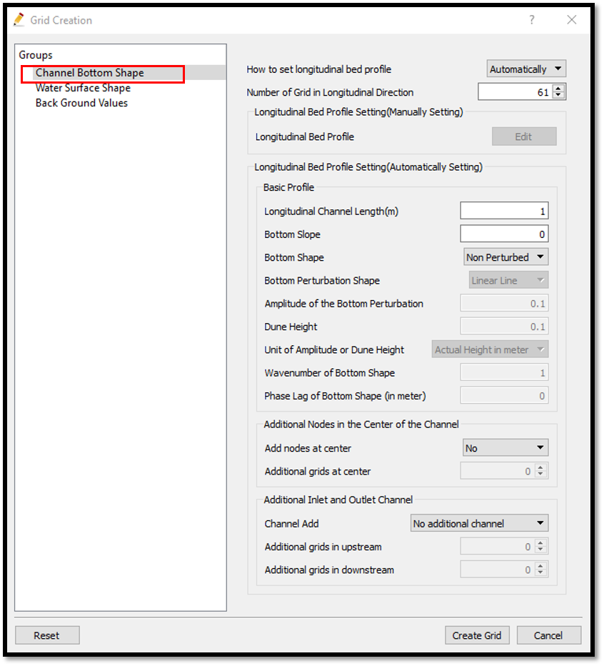
Figure 59 : Channel shape parameters
Give water surface shape parameters and no of grids in vertical direction as shown in Figure 60.
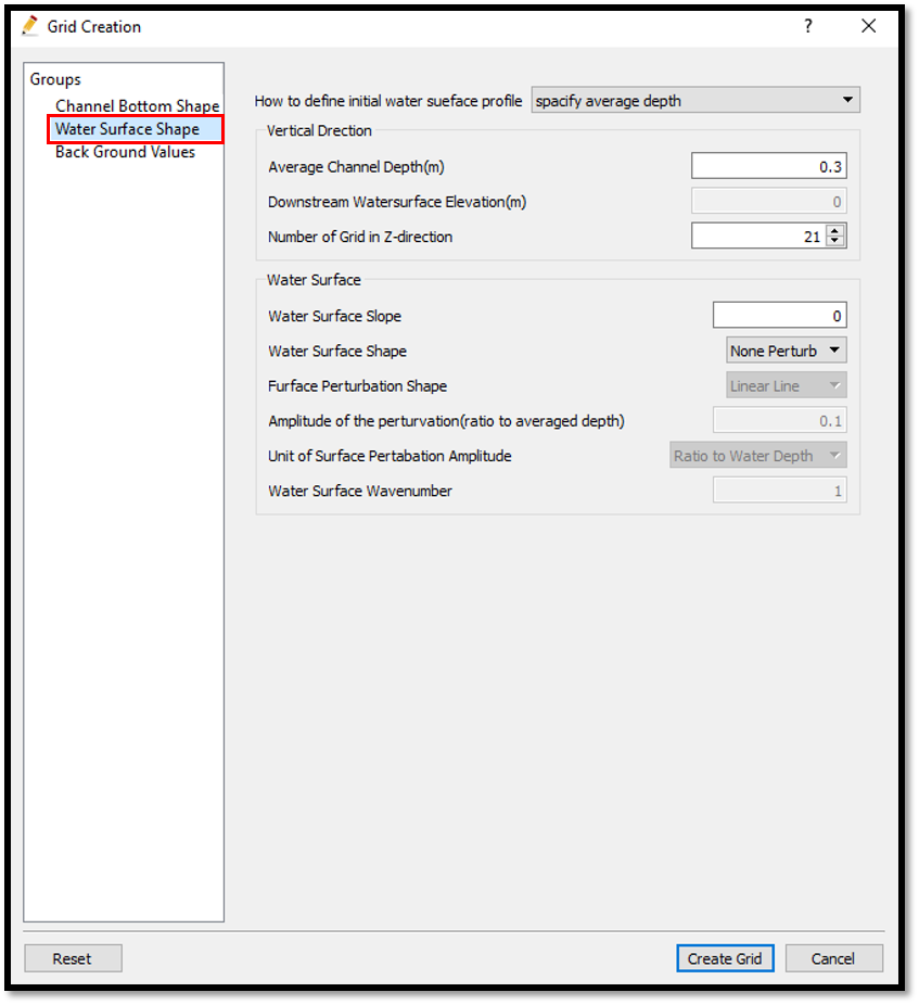
Figure 60 : Bottom and surface parameters
Give background values as shown in Figure 61.
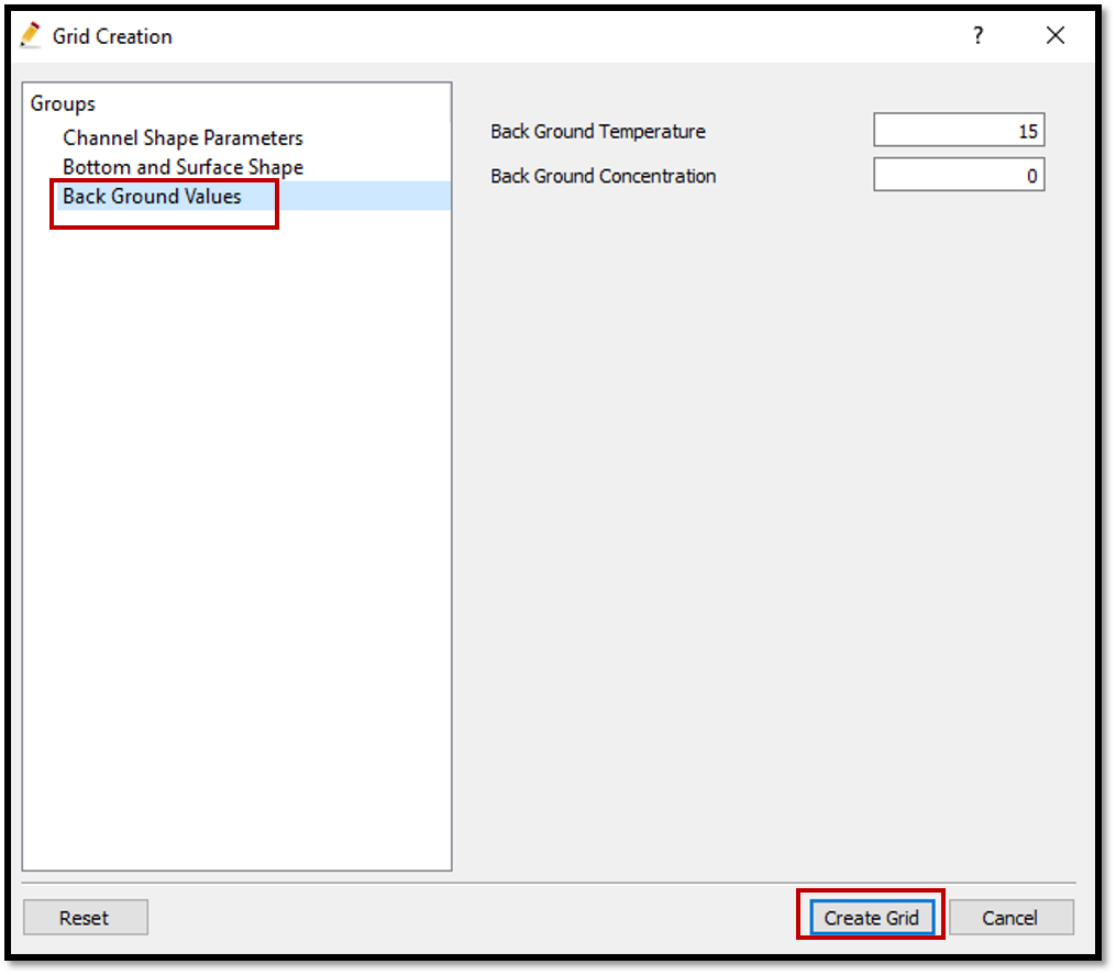
Figure 61 : Background values
For the background values, use 15 for background temperature and 0 for background concentration.
After giving the parameters for all the three main components, create the grid. After the grid creation, it will ask to map the geographic data to the grids. Select yes and it will map the conditions to the grids. After giving more conditions later you have to map those again.
Now the initial concentration has to be given in the vertical direction.
For that, add a polygon to initial concentration [Initial Concentration] [Add] [Polygon].
Then draw the polygon as shown in Figure 62.
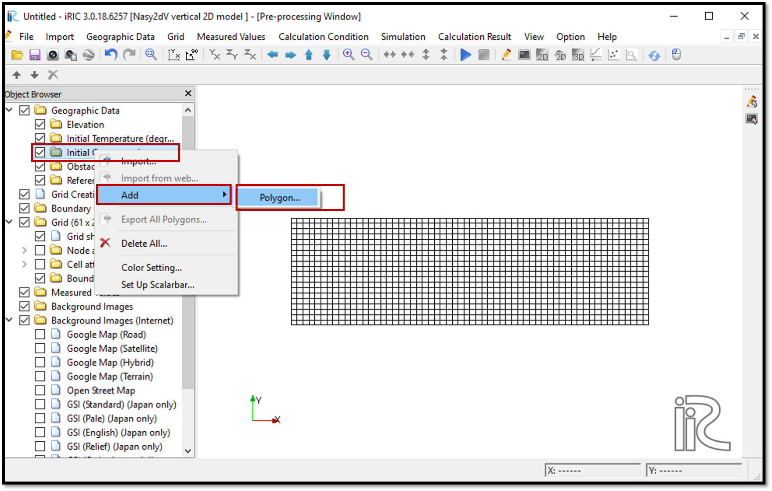
Figure 62 : Creation of initial concentration
Now draw the polygon in the upper middle area as shown in Figure 63.
Then give the value of initial concentration as 0.03 in this example. You can give your own values.
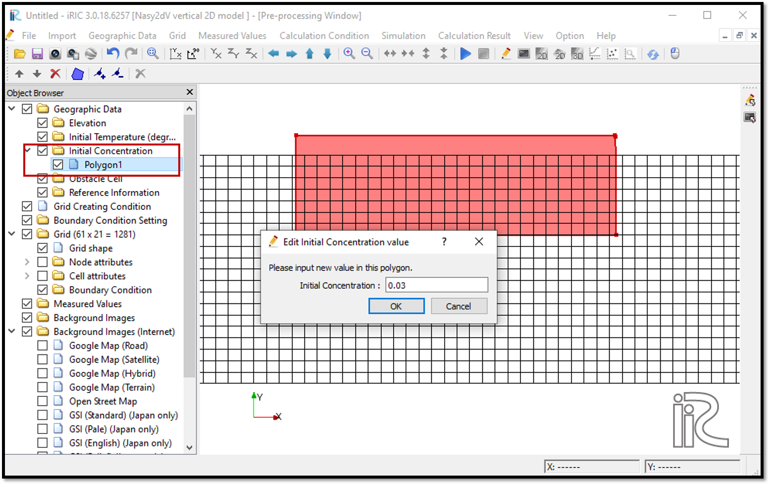
Figure 63 : Creation of initial concentration
After creating the initial concentration polygon, map it to the grids by , [Grids] [ Attributes Mapping] [Execute]. Then [Attribute Mapping] window will appear and tick on [Initial Concentration] and [OK] as shown in Figure 64.
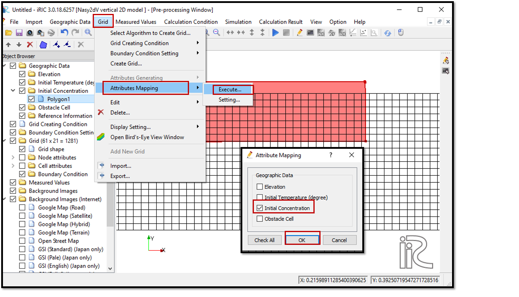
Figure 64 : Attributes mapping
Now the mapping is finished and it can be checked by ticking on [Grid][Cell Attributes][Initial Concentration].
Save the project [File][Save the Project as .ipro].
Setting the calculation conditions and simulation
The calculation conditions are given with, [Calculation Condition] [Setting]. Then the calculation condition window will appear.
Give computational parameters as shown in Figure 65.
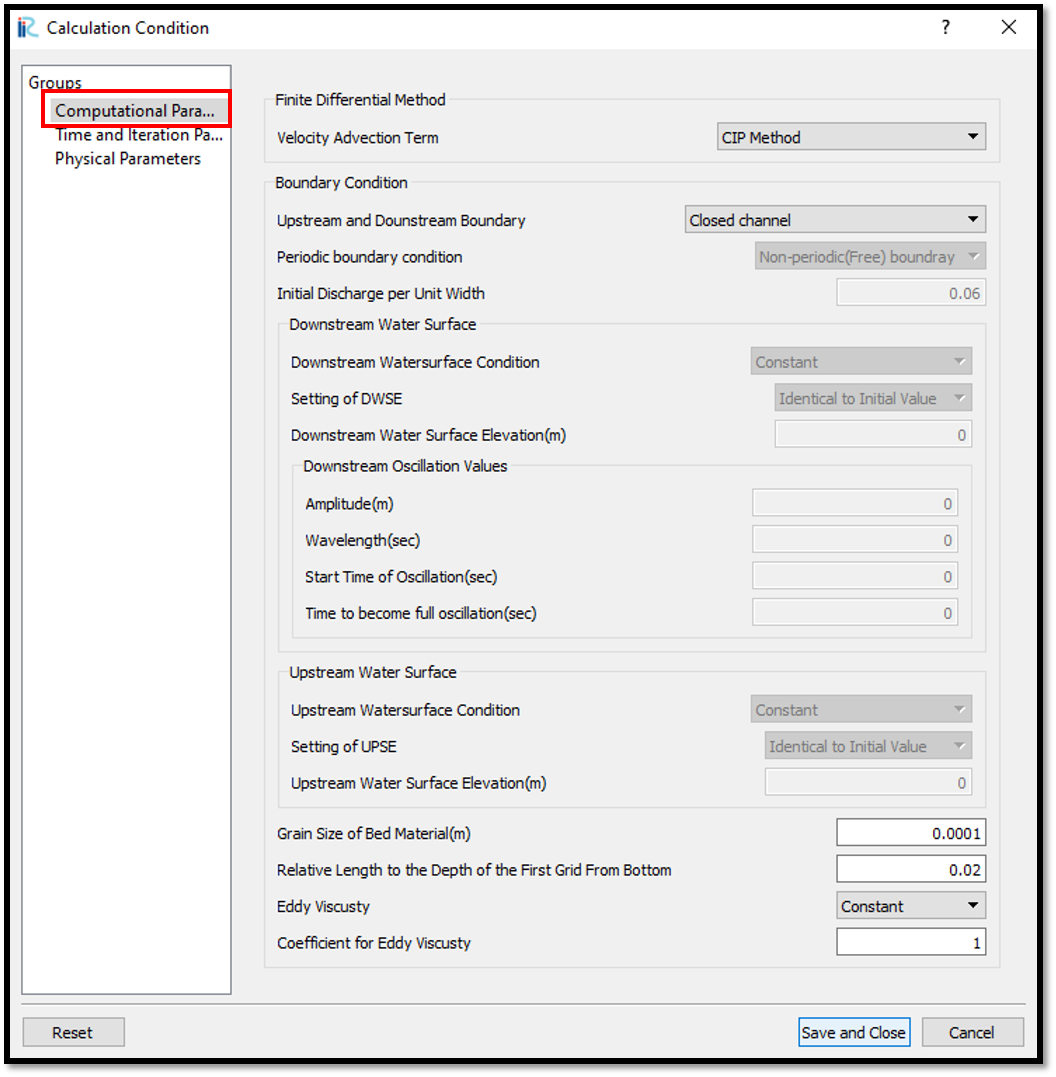
Figure 65 : Computational parameters
Give time and iteration parameters as shown in Figure 66.
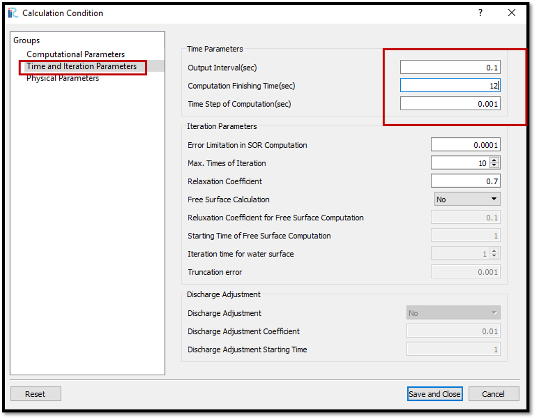
Figure 66 : Time and iteration parameters
Give physical parameters as shown in Figure 67.
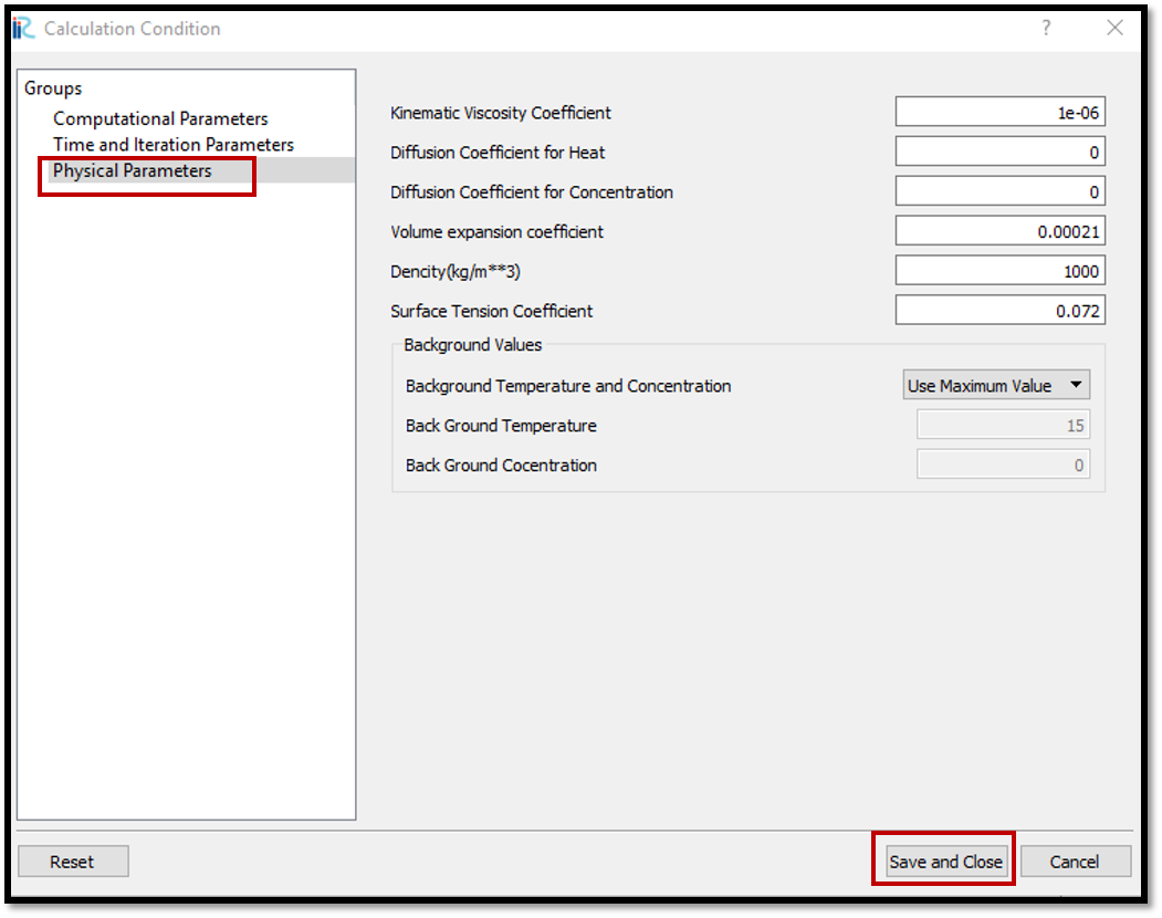
Figure 67 : Physical parameters
After giving the calculation conditions, [Save and close].
Save the whole project one more time with clicking on save icon and start to run the program by, [Simulation] [Run]. Program will start to run.
When the simulation finished, a dialogue box will appear with the message simulation stopped.
Visualization of results
Now go to icon or [Calculation Result][Open new 2D Post-Processing Window]. The 2D post processing window will appear.
You can tick on object browser for any parameter and adjust the properties by right clicking to visualize.
In this example we will see, [iRIC Zone] [Scaler] [Concentration].
Right click on [Concentration] and select [Property].
[Scaler setting] window will appear. Untick on [Automatic] in value range and give the values for minimum and maximum as shown in Figure 68.
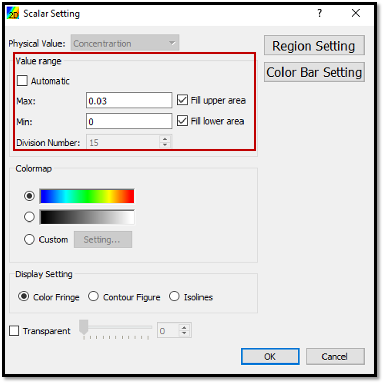
Figure 68 : Scaler setting
You can set the color maps as you like by selecting custom setting.
Adjust the color bar setting (i.e. fonts, position, size of the color bar etc) from the color bar setting tab and adjust the region by region setting tab.
To set the currents movements direction, select [Velocity] in object browser by ticking on [iRIC Zone] [Arrow] and [velocity].
Adjust the sizes of velocity vectors by right clicking on [Arrow] and selecting [Property].
The Figure 69 is the result of the above process.

Figure 69 : Concentration & velocity vector plot